Development of paper-based dual sensors
Paper-based sensors using Methyl Red (MR) and Bromocresol Purple (BCP) indicators were successfully developed. As shown in Fig. 2a,b, the MR sensors exhibited a pinkish-red coloration, while the BCP sensors appeared yellow under initial conditions. These sensors are pH-sensitive: an increase or decrease in pH causes the MR sensor to change from pinkish-red to yellow, whereas the BCP sensor transitions from yellow to purple. These color transitions are illustrated clearly in Fig. 3a,b.

(a) Methyl red (MR) sensor. (b) Bromocresol purple (BCP) sensor.

(a) Change in the MR sensor. (b) Change in the BCP sensor.
Fish packaging with different packaging techniques
After cleaning and filleting, all six varieties of fish were packaged using three different methods: conventional, vacuum, and shrink packaging. Low-Density Polyethylene (LDPE) and Polypropylene (PP) pouches were used for this purpose. Figure 4a,b,c show the packaging methods implemented.

(a) Conventional packaging. (b) Vacuum packaging. (c) Shrink packaging.
Colour analysis of the sensors
pH indicators used for monitoring the freshness of food typically alter their color in response to changes in the chemical composition of food samples during storage (Listyarini et al., 2018). Similarly, the color of paper-based dual sensors prepared using Methyl Red (MR) and Bromocresol Purple (BCP) indicators shifted when placed over fish samples stored under three different packaging conditions in refrigeration. To evaluate the effectiveness of these sensors, pH buffer solutions ranging from 3 to 7, with an incremental difference of 0.1, were prepared. These solutions were used to observe the corresponding color changes.
The results are presented in a graph, where the total color difference (dE) is plotted along the y-axis and the three different packaging configurations of the fish samples are plotted along the x-axis. Figure 5 illustrates the dE values of the MR sensor across different pH ranges, while Fig. 6 displays the dE values of the BCP sensor for the same pH ranges.

dE values of MR sensor at different pH range. Mean ± SD at p < 0.05 level for triplicate data.

dE values of BCP sensor at different pH range. Mean ± SD at p < 0.05 level for triplicate data.
As the pH levels in the package headspace increase during storage, volatile gases are released into the atmosphere (Fatemeh et al., 2017). Consequently, the color of the sensors changes, indicating the freshness of each sample. The findings reveal that the total color difference is more pronounced in the pH range between 4 and 6 compared to other ranges. The data further suggest that the sensors become darker as the pH approaches a more basic state, causing the color of the indicators to change accordingly.
The color of both sensors placed over the fish samples for a period of 12 days, with observations recorded at 3-day intervals, indicated that the overall color change in the sensors for Mackerel, Sardine, Cuttlefish, and Pomfret samples was relatively higher compared to Prawn and Red Snapper.
Figure 7 presents the dE values against the pH values for the MR and BCP sensors attached to vacuum-packed Sardine and Mackerel samples stored at refrigerated temperatures. Figure 8 illustrates the dE values against the pH values for MR and BCP sensors attached to vacuum-packed Prawn and Cuttlefish samples under the same storage conditions. Similarly, Fig. 9 displays the dE values against the pH values for MR and BCP sensors linked to vacuum-packed Red Snapper and Pomfret samples kept at refrigerator temperature.

dE values of MR and BCP sensors attached with sadrine and mackerel stored at refrigerator temperature.

dE values of MR and BCP sensors attached with prawn and cuttle fish stored at refrigerator temperature.

dE values of MR and BCP sensors attached with Red snapper and Pomfret stored at refrigerator temperature.
Estimation of pH
After the death of the fish, blood circulation halts, cutting off its oxygen supply. As a result, enzymes in the muscle break down glycogen into its component molecules, producing lactic acid. This process causes a decline in the pH of the fish muscle. The production of lactic acid continues until the glycogen supply is completely exhausted. Following this stage, rigor mortis sets in, characterized by muscle stiffness, which is then gradually followed by a decrease in stiffness and an increase in pH, leading to muscle softening (Tavares et al., 2021).
Data collected and presented in Table 1 shows that on the zeroth day (immediately after harvest), the pH was approximately 7, indicating that the fish was freshly caught and retained a high level of nutritional value. Fresh fish typically have a pH range of 6.0 to 6.5, characterized by firm flesh and no foul smell. Moderately fresh fish exhibit a pH range of 6.5 to 6.8, with a softer texture and mild odor, but are still considered edible. In contrast, spoiled fish have a pH greater than 6.8, sometimes exceeding 7.5, accompanied by a slimy texture and a strong ammonia-like odor. This correlation between fish freshness and pH during cold storage was also reviewed by Abbas et al.19.
As the number of storage days increased, the pH initially decreased but then began to rise gradually. This is attributed to the emission of TVB-N, which is accompanied by the production of alkaline bacterial metabolites19.
Estimation of protein
Fish, particularly Mackerel, Sardine, and Pomfret, are well-known for their high protein content. To quantify the protein levels in fresh fish samples, Lowry’s method was employed, and the results are presented in Table 2. When the experiment was repeated at 3-day intervals, it was observed that the protein content gradually decreased over time. This decline was not abrupt but progressive. The reduction in protein levels is primarily attributed to autolysis, an intrinsic breakdown of proteins and fats caused by a series of complex enzyme reactions.
Since the samples were stored under refrigerated conditions, the rate and extent of protein degradation were significantly minimized. Shenouda et al. (1980) demonstrated that several factors contribute to protein loss in fish during refrigeration, including enzyme-mediated activity of trimethylamine oxide (TMAO), an increase in solute concentration, dehydration, the formation of ice crystals, and accretion.
Estimation of fat
Hydrolysis and oxidation are two distinct chemical reactions that occur during the processing and storage of fish, both contributing to the reduction of fat content. During lipid hydrolysis, free fatty acids are released, leading to the denaturation of proteins as their structure is compromised (Bashir et al., 2021). It was observed that the fat content decreased progressively as the storage period increased.
After being refrigerated for 12 days, the fat content in the fatty fish Mackerel and Sardine dropped from 12 to 9 g and 11 to 9 g, respectively. A similar trend was observed in the other four fish samples: Red Snapper, Cuttlefish, Pomfret and Prawn. The results are summarized in Table 3. The reduction in lipid content during refrigerated storage is primarily attributed to oxidation. This oxidative reaction generates peroxides, which accelerate the degradation of fish quality (A. Keyvan et al., 2008).
Results of random forest model
The random forest model was trained using data collected from six different varieties of fish, each packed using different packaging methods. Table 4 presents the observed values for L*, a*, b*, dE, pH, protein and fat over a period of 0 to 12 days under refrigerated conditions.
The random forest model was trained separately for each variety of fish. The decision tree generated for the Prawn variety is shown in Fig. 10. The decision tree possesses several essential characteristics that define its structure and functionality. At the root node, the initial condition is established as protein ≤ 11.775, which splits the dataset into two branches: the left branch if the condition is true, and the right branch if it is false. Intermediate nodes further refine the data subsets. For example, in the left subtree, further divisions occur based on criteria such as package ≤ 0.5. Similarly, the right subtree branches off according to parameters like TVB-N ≤ 11.32 and dE ≤ 34.73.
Decision tree from random forest for prawn.
Leaf nodes, represented as terminal boxes, indicate the final predictions of the tree. Each node in the tree displays the number of samples that reach that specific point. Additionally, the squared error at each node serves as a measure of predictive accuracy, where smaller values signify better performance.
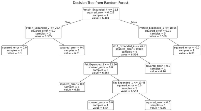
The random forest model was trained separately for each variety of fish. The decision tree generated for the fish variety Pomfret is shown in Fig. 11. This decision tree possesses several key characteristics that define its structure and functionality. At the root node, the initial condition is established as protein ≤ 14.175, which divides the dataset into two branches: the left branch if the condition is true and the right branch if it is false. Intermediate nodes further refine the data subsets. For example, in the left subtree, additional splits occur based on criteria such as TVB-N ≤ 15.035. Similarly, in the right subtree, divisions are made according to parameters like dE ≤ 28.66.
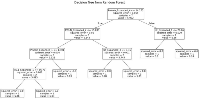
Decision tree from random forest for Pomfret.
Leaf nodes, represented as terminal boxes, indicate the final predictions of the tree. These leaf nodes mark the completion of the decision-making path, where the model assigns a prediction based on the features observed.
The random forest model was trained separately for each variety of fish. The decision tree generated for the fish variety Red Snapper is shown in Fig. 12. This decision tree possesses several key characteristics that define its structure and functionality. At the root node, the initial condition is established as protein ≤ 21.77, which divides the dataset into two branches: the left branch if the condition is true and the right branch if it is false. Intermediate nodes further refine the data subsets. For example, in the left subtree, additional splits occur based on criteria such as TVB-N ≤ 11.815. Leaf nodes, represented as terminal boxes, indicate the final predictions of the tree. These leaf nodes mark the end of the decision-making path, where the model makes its final prediction based on the observed features.
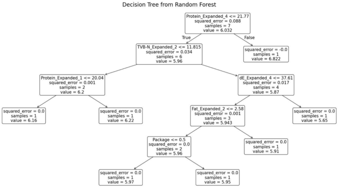
Decision tree from random forest for red snapper.
The random forest model was trained separately for each variety of fish. The decision tree generated for the fish variety Sardine is shown in Fig. 13. This decision tree possesses several key characteristics that define its structure and functionality. At the root node, the initial condition is established as fat ≤ 12.545, which divides the dataset into two branches: the left branch if the condition is true and the right branch if it is false. Intermediate nodes further refine the data subsets. For example, in the left subtree, additional splits occur based on criteria such as TVB-N ≤ 23.715. Similarly, the right subtree is divided according to parameters like TVB-N ≤ 18.08. Leaf nodes, represented as terminal boxes, indicate the final predictions of the tree. These leaf nodes mark the conclusion of decision paths, where the model outputs its final prediction based on the observed features.
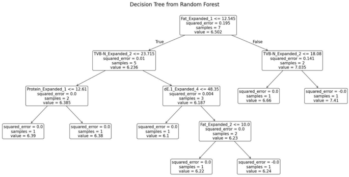
Decision tree from random forest for sardine.
The random forest model was trained separately for each variety of fish. The decision tree generated for the fish variety Mackerel is shown in Fig. 14. This decision tree possesses several key characteristics that define its structure and functionality. At the root node, the initial condition is established as protein ≤ 9.84, which divides the dataset into two branches: the left branch if the condition is true and the right branch if it is false. Intermediate nodes further refine the data subsets. For example, in the left subtree, additional splits occur based on criteria such as TVB-N ≤ 22.67. Similarly, the right subtree is divided according to parameters like dE ≤ 28.83. Leaf nodes, represented as terminal boxes, indicate the final predictions of the tree. These leaf nodes mark the end of decision paths, where the model outputs its final prediction based on the observed features.
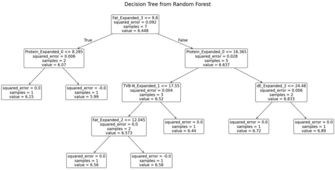
Decision tree from random forest for mackerel.
The random forest model was trained separately for each variety of fish. The decision tree generated for the fish variety Cuttlefish is shown in Fig. 15. This decision tree exhibits several key characteristics that define its structure and functionality. At the root node, the initial condition is set as TVB-N ≤ 22.23, which divides the dataset into two branches: the left branch if the condition is true and the right branch if it is false. Intermediate nodes further refine the data subsets. For example, in the left subtree, additional splits occur based on criteria such as fat ≤ 3.125. Leaf nodes, represented as terminal boxes, indicate the final predictions of the tree. These leaf nodes mark the end of decision paths, where the model outputs its final prediction based on the observed features.
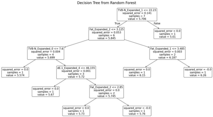
Decision tree from random forest for Cuttle fish.
The random forest model generates multiple decision trees during the training phase. When testing the model, an unknown sample is provided, and the model predicts its pH value. The performance of the random forest model is assessed using evaluation metrics such as Mean Absolute Error (MAE), Mean Squared Error (MSE), and Root Mean Squared Error (RMSE). Table 5 presents the predicted pH values alongside the corresponding evaluation metrics.
The freshness of the fish is classified into three categories namely Fresh, Moderately Fresh, and Spoiled based on the predicted pH values using the trained Random Forest model. The freshness category for each fish type on the 15th day of vacuum storage is shown in Table 6.
