Overview of survivalFM
Figure 1 presents an overview of survivalFM. We developed survivalFM to estimate all potential pairwise interaction effects among input variables for right-censored survival data, such as time to disease onset. It is based on the widely utilized proportional hazards model1 which associates time-to-event outcomes with a set of predictor variables through a hazard function of the form:
$$h(t| {{{\bf{x}}}})={h}_{0}(t)\exp (\;f({{{\bf{x}}}}))$$
(1)
where h(t∣x) represents the hazard for an individual at time point t, with the baseline hazard function h0(t) describing the time-varying hazard and the partial hazard \(\exp (f({{{\bf{x}}}}))\) quantifying the impact of the predictor variables x on the baseline hazard. In the standard formulation of the Cox proportional hazards model, the partial hazard \(\exp (f({{{\bf{x}}}}))\) is assumed to be parametrized by a linear combination of the predictor variables f(x) = β⊤x, with β giving the weights for the individual variables.
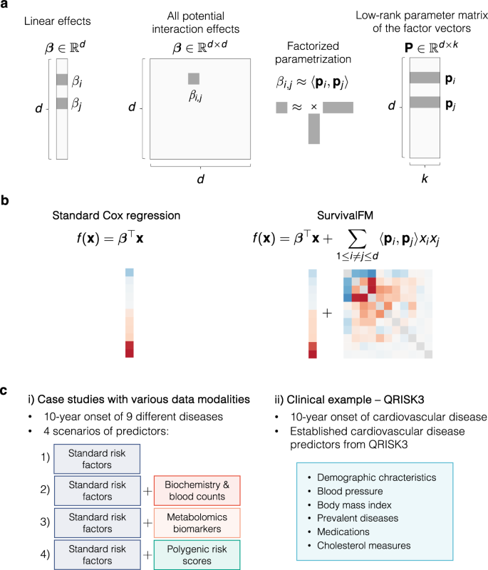
a A machine learning survival analysis method, survivalFM, is developed to estimate linear and all pairwise interaction effects between predictor variables using factorized parametrization of the interaction terms βi,j ≈ 〈pi, pj〉. d denotes the number of predictor variables and k is a hyperparameter defining the rank of the factorization of the interaction terms. Typically, the rank of the factorization is substantially lower than the number of predictor variables (k ≪ d), which allows interaction effects to be computed efficiently even with high-dimensional input data. b The added value of incorporating comprehensive interaction terms using survivalFM is assessed by comparing its performance to the standard linear Cox proportional hazards regression. f (x) parameterizes the partial hazard function in a proportional hazards model \(h(t| {{{\bf{x}}}})={h}_{0}(t)\exp (\;f({{{\bf{x}}}}))\). c The performance is evaluated in various disease prediction examples: i) case studies with four different predictor sets, each applied to nine disease examples; ii) a clinical example using predictors from the QRISK3 cardiovascular disease (CVD) risk evaluation tool.
In many applications, understanding how variables may interact to jointly impact the hazard rate can provide additional value beyond their independent linear effects. However, directly fitting all potential pairwise interaction effects in a multivariable prediction model quickly becomes challenging due to the quadratic increase in the number of interaction terms as a function of the number of input variables. Hence, we propose survivalFM, an extension which adds an approximation of all pairwise interaction effects using a factorized parametrization approach (Fig. 1a-b):
$$f({{{\bf{x}}}})={{{{\boldsymbol{\beta }}}}}^{\top }{{{\bf{x}}}}+{\sum}_{1\le i\ne j\le d}{\widetilde{\beta }}_{i,j}{x}_{i}{x}_{j}={{{{\boldsymbol{\beta }}}}}^{\top }{{{\bf{x}}}}+{\sum}_{1\le i\ne j\le d}\langle {{{{\bf{p}}}}}_{i},{{{{\bf{p}}}}}_{j}\rangle {x}_{i}{x}_{j}$$
(2)
where 〈 ⋅ , ⋅ 〉 denotes the inner product and d denotes the number of predictor variables. The first part contains the linear effects of all predictor variables in the same way as in the standard formulation of the Cox proportional hazards model. The second part contains all pairwise interaction effects between the predictor variables xi and xj. However, instead of directly estimating the interaction effects βi, j, the effects are approximated through a factorized parameterization using an inner product between two low-rank latent vectors \({\widetilde{\beta }}_{i,j}=\langle {{{{\bf{p}}}}}_{i},{{{{\bf{p}}}}}_{j}\rangle\). The parameter vectors \({{{{\bf{p}}}}}_{i}\in {{\mathbb{R}}}^{k}\) and \({{{{\bf{p}}}}}_{j}\in {{\mathbb{R}}}^{k}\) are the row vectors of a low-rank parameter matrix \({{{\bf{P}}}}\in {{\mathbb{R}}}^{d\times k}\) (Fig. 1a). Hence, this results in much fewer parameters to estimate, as the rank used in the factorization is typically substantially lower than the total number of predictor variables (k ≪ d). With this approach, we avoid the statistical and computational problems that would be encountered with direct estimation of all interactions terms in the presence of many predictor variables, while still maintaining interpretability. The idea of using factorized parametrization strategy originates from factorization machines (FMs)11, originally proposed for regression and classification tasks in the context of recommender systems. For more details of the model and the fitting procedure, see Methods.
Study population, disease outcomes and data modalities
To evaluate whether survivalFM could improve risk prediction models and provide new insights into the joint effects of risk factors on disease onset, we performed analyses using data from the UK Biobank. This cohort comprises a total of ~500,000 participants from the UK, enrolled in 21 recruitment centers across the country. Upon agreeing to participate, individuals visited the nearest assessment center to provide baseline data, physical measurements, and biological samples.
Of the entire UK Biobank cohort, 93% of participants were recruited in assessment centers located in England and Wales, and 7% in Scotland. Previous studies have revealed differences in health-related characteristics between these regions12,13. Given these regional differences and following approaches used in other prediction studies in UK Biobank12,14,15, we trained our models using data collected from participants enrolled in England and Wales and tested them using data from participants enrolled in Scotland.
The UK Biobank is renowned for its comprehensive phenotyping and molecular profiling, including routine blood biomarkers and advanced ’omics measurements such as genomics and metabolomics. Baseline characteristics of the study population and a summary of the datasets studied here are summarized in Supplementary Data 1. As disease outcomes, we considered the 10-year incidence of nine example diseases, selected to comprise common diseases and diseases which can benefit from intervention if identified early (Supplementary Data 2 and 3). Disease endpoints were defined based on hospital episode statistics, death registries, self-reported outcomes, and, where available, primary care data (Methods). For lung cancer, we additionally incorporated data from the cancer registry. Prevalent cases were defined as individuals with a recorded first occurrence of a given outcome before the baseline assessment visit and were excluded from analyses for each respective disease endpoint.
To assess the performance across different data modalities, we considered four different prediction scenarios that incorporate an array of predictors ranging from traditional clinical predictors to more advanced omics-based data sources (Fig. 1c, Methods). In the first scenario, we started from a set of standard cardiovascular risk factors included in the ASCVD risk estimator plus16, widely recognized in various primary prevention scores. Since these factors have been shown to be predictive beyond cardiovascular diseases17,18,19, we included them as standard risk factors across all analyzed disease examples. We then added sets of more complex data layers to these standard risk factors (Fig. 1c). In the second scenario, we added a comprehensive set of hematologic and clinical biochemistry measures to the standard risk factors; in the third scenario, we incorporated a wide range of metabolomic biomarkers, recently shown promise as an assay to inform on multidisease risk17,20; and finally, we included a set of polygenic risk scores for both disease and quantitative traits21, which have gained interest for their potential to enhance risk prediction models by providing complementary information to traditional risk factors22,23,24.
survivalFM improves risk prediction across diverse diseases and data modalities
The practical utility of any risk prediction model is determined by its ability to stratify risk and identify high-risk individuals. We evaluated the ability of survivalFM to predict future disease risk and benefit from the comprehensive interaction terms by comparing its performance to standard linear Cox proportional hazards regression (Fig. 1b), employing L2 (Ridge) regularization in both methods to control model complexity and prevent overfitting (Methods). Regularization parameters were optimized via 10-fold cross-validation within the training set (England and Wales participants), selecting the values that maximized the concordance index (C-index) across validation folds. The final obtained models were then tested on the participants enrolled in Scotland.
By modeling the comprehensive interactions present in the underlying data, survivalFM improved the discriminatorion performance across a majority of the studied examples, as measured by concordance index (C-index; Fig. 2). Specifically, statistically significant improvements were noted in 11 of the 36 evaluated scenarios (30.6%), with a mean improvement in C-index (ΔC-index) of 0.0054. Minor improvements were noted in another 23 of the 36 of scenarios (63.9%), with a mean ΔC-index of 0.0014. Importantly, none of the studied examples demonstrated a statistically significant decrease in performance with survivalFM, highlighting its robustness. Absolute values for the C-indices are detailed in Supplementary Data 4, demonstrating good discriminative performance across all models with C-indices ranging from 0.68 to 0.92.
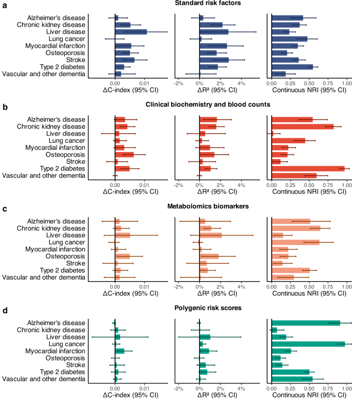
Comparison of the predictive performance of survivalFM to standard linear Cox proportional hazards regression in terms of improvements in concordance index (ΔC-index), Royston’s R2 (ΔR2) and continuous net reclassification (NRI). Results are shown for nine disease examples (y-axis) across four data modalities, computed for individuals in the Scotland test set: a standard risk factors (blue; included in all models), b clinical biochemistry and blood counts (red), c metabolomics biomarkers (orange) and d polygenic risk scores (green). Bars represent the observed value of the model performance metric; horizontal error bars denote 95% confidence intervals (CIs), estimated with bootstrapping over 1000 resamples. Sample sizes and event counts for each disease example are provided in Supplementary Data 3. Source data are provided as a Source Data file.
We further evaluated performance of the models using Royston’s R225 (Fig. 2), which extends the concept of explained variation to survival outcomes, providing a measure of overall model fit. In terms of R2, statistically significant increases in the proportion of explained variation were observed in 15 of the 36 examples (41.67%), with a mean R2 improvement (ΔR2) of 1.62 percentage points. Minor improvements were observed in 17 of the 36 examples (47.2%), with a mean improvement of 0.53 percentage points. None of the studied examples demonstrated a statistically significant reduction in the explained variation with survivalFM. Absolute R2 values are detailed in Supplementary Data 4, with the proportion of explained variation across the examples ranging from 24.9% to 95.0%.
Given that even modest improvements in discrimination performance at the population level can substantially affect individual risk predictions, we also evaluated model performance using continuous net reclassification improvement (NRI), which has been shown to provide complementary information on risk model performance26,27. The continuous NRI quantifies the extent to which the model appropriately increases the predicted probabilities for subjects who experience events and decreases them for those who do not. This metric is particularly useful in the absence of established clinical thresholds for high-risk groups, as it quantifies the improvement in risk prediction without relying on predefined risk cutoffs and thus facilitates comparisons across different diseases.
In terms of continuous NRI, survivalFM yielded significantly improved resclassification in 34 of 36 (94.4%) of the studied examples, with a mean continuous NRI of 0.41. Minor improvements were noted in the remaining 2 of the 36 examples, with a mean continuous NRI of 0.046. Therefore, despite the relatively modest improvement magnitudes in the C-indices, the continuous NRI indicated notable positive changes in individual risk predictions. For instance, type 2 diabetes modeled using clinical biochemistry and blood counts data demonstrated the highest continuous net reclassification improvement of 0.97 (95% CI 0.91–1.03), corresponding to 34% (95% CI 28–40%) of events and 63% (95% CI 62–64%) of non-events having improved risk estimates (Fig. 3).
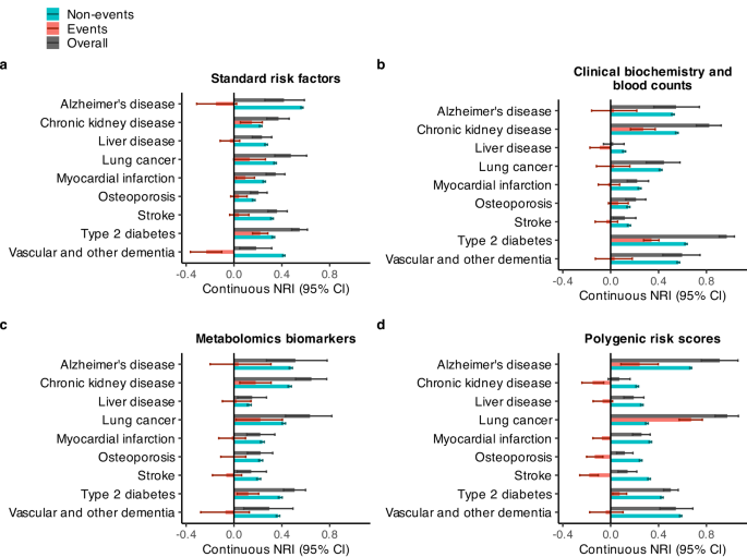
Continuous net reclassification improvements (NRI) (in dark gray), separated by events (red) and non-events (blue). Results are shown for nine disease examples (y-axis) across four data modalities: a standard risk factors (included in all models), b clinical biochemistry and blood counts, c metabolomics biomarkers, and d polygenic risk scores, computed for individuals in the Scotland test set. Bars represent the observed value of the model performance metric; horizontal error bars denote 95% confidence intervals (CIs), estimated with bootstrapping over 1000 resamples. Sample sizes and event counts are provided in Supplementary Data 3. Source data are provided as a Source Data file.
To further elucidate the components of the net reclassification improvements, we examined the continuous NRI separately for individuals who experienced events and those who did not (Fig. 3). While the overall continuous NRI was positive across all studied examples, the relative contributions of event- and non-event-specific reclassification varied across diseases and data modalities. Among individuals who experienced events, statistically significant improvements in NRIevents were observed in 11 out of 36 examples (30.6%), with a mean improvement of 0.235. Minor improvements in NRIevents were noted in 9 of the 36 examples (25.0%), with a mean improvement of 0.047. Conversely, statistically significant decreases in NRIevents were observed in 6 out of 36 examples (16.7%), with a mean reduction of 0.143. However, even in these cases, the overall NRI remained positive due to substantial improvements in NRInon-events. Among individuals who did not experience events, the NRInon-events demonstrated statistically significant improvements across all studied examples. Furthermore, in scenarios where NRIevents was negative, the decrease was smaller in magnitude compared to the corresponding gains in NRInon-events, resulting in a positive overall NRI.
To evaluate whether the presence of genetically related individuals between the training and test sets influenced predictive performance, we performed an additional sensitivity analysis. Specifically, we excluded from the Scotland test set all individuals who were genetically related to any member of the England and Wales training set. We defined relatedness as third-degree or closer relatives, using a kinship coefficient threshold of ≥0.044228. Under this more stringent exclusion criterion, the predictive performance of survivalFM remained stable, with only minor numerical fluctuations and no meaningful reduction in the performance metrics (Supplementary Figs. 5, 6). These findings indicate that observed predictive performance is not influenced by the inclusion of related individuals in the test set.
Overall, the models demonstrated good calibration in the Scotland test set, with the exception of chronic kidney disease (Supplementary Figs. 1–4). In this case, both standard Cox regression and survivalFM models trained on the England and Wales training set systematically overestimated disease risk in the Scotland test set across all input types, likely due to differences in chronic kidney disease incidence rates between Scotland and England and Wales in the UK Biobank (Supplementary Data 3).
In addition to our primary analyses, we conducted a supplementary analysis combining all the input data types (standard risk factors, clinical biochemistry and blood counts, metabolomics biomarkers, and polygenic risk scores). This analysis was restricted to individuals in the UK Biobank who had measurements available for all these data types; baseline characteristics, sample sizes, and event counts for this combined analysis are detailed in Supplementary Data 5, 6. In this combined model, the performance gains from modeling comprehensive interactions remained largely consistent but were slightly attenuated (Supplementary Fig. 7), likely due to the increased number of predictor variables, some of which may already capture associations that overlap with the interaction effects. Specifically, in terms of discrimination, minor but statistically non-significant improvements in C-index were observed in 7 out of 9 examples (77.8%), with a mean ΔC-index of 0.0016. For Royston’s R2, a statistically significant increase was noted in one example (chronic kidney disease, ΔR2 = 1.16 percentage points), while minor improvements were present in 4 out of 9 examples (44.4%), with a mean ΔR2 of 0.23 percentage points. Despite the modest improvements in discrimination and explained variation, continuous NRI demonstrated more pronounced effects: statistically significant improvements were observed in 6 out of 9 examples (66.7%), with a mean NRI of 0.652, while minor improvements were noted in 2 out of 9 examples (22.2%), with a mean NRI = 0.0472.
These findings suggest that interaction terms carry additional predictive information across various disease and data modalities and survivalFM can model this residual contribution. While the extent of improvement varied depending on the specific disease and dataset under study, improvements were consistently observed across multiple disease areas and data types.
Disease-specific interaction profiles
A key advantage of survivalFM is that despite introducing a more complex layer of non-linearity through the interaction terms, it still maintains interpretability and transparency of how the model predictions are made. To compare the interactions identified by survivalFM with those detected using a conventional approach of explicitly enumerating them in a standard Cox regression model, we performed additional analyses by fitting Cox models with all possible pairwise interactions explicitly included (Methods). Due to computational constraints, this analysis was limited to the standard risk factor dataset with the fewest input predictors.
Despite differences in model parameterization and optimization, both approaches for modeling interactions yielded similar improvements in predictive performance (Supplementary Fig. 8). Furthermore, a comparison of the estimated coefficients (for both main and interaction effects) between survivalFM and Cox regression showed strong concordance (Supplementary Fig. 9). Model predictions were nearly identical, with correlation coefficients exceeding 0.99 in all cases (Supplementary Fig. 10). These findings indicate that, despite methodological differences, both approaches produce highly comparable results. Practically, this suggests that the interaction coefficients in survivalFM (βij = 〈pi, pj〉) can be interpreted similarly to those in a standard Cox model (βij). Thus, survivalFM maintains the interpretability of interaction effects while offering a more compact representation that mitigates the computational burden associated with estimating numerous interactions simultaneously.
Analysis of the estimated interaction effects from survivalFM across the studied disease outcomes and different input datasets revealed that in many cases there was a diverse interaction landscape contributing to these predictions, demonstrating that the observed performance gains are likely to stem from the cumulative benefit of many small interaction effects rather than a few prominent ones (examples shown in Supplementary Figs. 11–13). Here, we will highlight a few examples with some of the most notable performance gains.
Including interaction terms significantly improved predictive performance across various diseases, with liver diseases modeled using standard risk factors or metabolomic biomarkers being among those showing the highest gains in C-index and R2 (Fig. 2). In the liver disease model based on standard risk factors, prominent interactions emerged among different cholesterol measures, cholesterol-lowering medication, age, body mass index, and sex (Supplementary Fig. 11). These results suggest that the joint effects of these risk factors further explain the risk of chronic liver disease outcomes beyond their additive linear effects. Additionally, smoking status was highly weighted both individually and in the interactions, aligning with the earlier research suggesting that smoking may exacerbate the influence of the other risk factors in the development of chronic liver diseases29. In the liver disease model based on metabolomics (Supplementary Fig. 12), various measures of lipid subclasses were highly weighted as individual predictors, while interactions especially among various amino acids were prominent, aligning with previous research on altered amino acid metabolism in chronic liver disease30,31. Acetate exhibited a notably strong interaction profile, consistent with its established role in alcohol metabolism and lipid accumulation in the liver32,33.
A contrasting example was type 2 diabetes modeled using clinical biochemistry and blood counts data, which obtained the highest observed continuous NRI. Unlike the other examples, analysis of the model coefficients revealed that the model weights were predominantly concentrated around glycated hemoglobin (HbA1c) and its interactions across the other variables (Supplementary Fig. 13). The highest interaction weight was attributed to the interaction between HbA1c and glucose, which was negatively weighted despite their positive individual effects. This likely reflects the fact that the simultaneous elevation of both HbA1c and glucose does not increase risk additively but rather relates to them being correlated measures of blood glucose regulation and overall glycemic control. Additionally, the model highlighted positively weighted interactions of HbA1c with age, white ethnicity, and urate levels, indicating these factors together might amplify the risk. In contrast, interactions between HbA1c and reticulocyte count and body mass index were negatively weighted.
survivalFM benefits from large training data sizes
To understand the impact of training data size on model performance and the ability of survivalFM to leverage interaction terms, we conducted analyses with models trained on varying-sized subsets of the training data. Throughout these analyses, the Scotland test set remained fixed, allowing us to analyze how changes only in the number of training individuals influence model performance. Figure 4 shows the discrimination performance of survivalFM as a function of the number of training individuals for the input dataset involving standard risk factors (results for the other predictor sets are shown in Supplementary Figs. 14–16). For the standard risk factor input dataset (Fig. 4), which contains the fewest predictors and therefore permits feasible inclusion of all pairwise interaction terms, we also include a Cox model with interaction terms as a reference. This provides additional context by serving as a benchmark for performance when interactions are explicitly modeled using a standard approach. These results demonstrate a clear dependency on large sample sizes to uncover predictive interaction terms, with survivalFM generally requiring at least 50,000 individuals in training to outperform standard Cox regression. The discriminatory performance of survivalFM shows a positive trend and increasing gap to standard Cox regression with increasing sample sizes, although the gains often begin to plateau at the upper end of the sample size range.
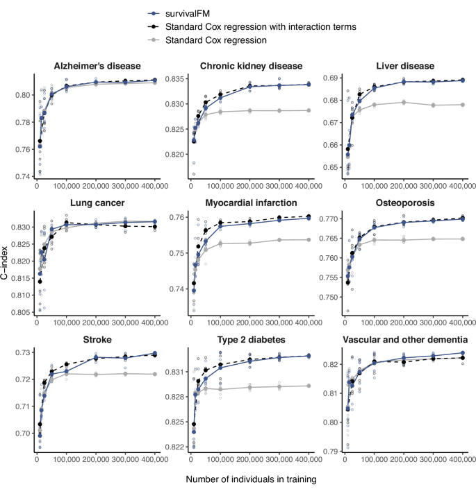
Impact of the size of the training dataset (x-axis) on the discrimination performance in the Scotland test, measured by concordance index (C-index; y-axis), comparing survivalFM (blue, solid line) to standard Cox regression (gray, solid line) and standard Cox regression incorporating all pairwise interactions (black, dashed line). Results are shown for the input dataset consisting of standard risk factors. For each training dataset size, the analysis was repeated five times by randomly sampling with replacement from the full training set. Hollow points indicate the performance from each individual iteration, while filled points (connected by lines) show the average performance. Sample sizes and event counts for each example are provided in Supplementary Data 3. Source data are provided as a Source Data file.
survivalFM improves prediction performance in a clinical cardiovascular risk prediction scenario
To explore whether comprehensive interaction modeling via survivalFM could also refine well-established clinical risk prediction models, we conducted analyses in a clinical CVD risk prediction setting using predictors from the QRISK3 model5. QRISK models are Cox proportional hazard models used for predicting the patient’s 10-year risk of CVD, recommended by the healthcare guidelines in the UK. The latest version, QRISK3 from 20175, incorporates a variety of risk factors and comorbidities, along with a set of their interaction terms with age.
We aimed to determine if comprehensive modeling of the interaction terms among the QRISK3 risk factors using survivalFM could improve the model’s ability to predict cardiovascular risk. The endpoint was defined as 10-year incidence of composite CVD, including coronary heart disease, ischemic stroke, and transient ischemic attack, and including both fatal and non-fatal events (Supplementary Data 7, Methods). Following the exclusion criteria from the QRISK3 derivation study, we excluded participants with prior CVD diagnoses and those on a cholesterol-lowering medication at the study entry. The baseline characteristics of the study population in this clinical prediction scenario are detailed in Supplementary Data 8.
To ensure a fair comparison of the models, we retrained the QRISK3 model in the UK Biobank considering the same set of risk factors (Methods). As prior research has shown QRISK3 to systematically overestimate CVD risk in the UK Biobank34, retraining the model ensures an accurate calibration for this cohort. We evaluated three models of increasing complexity: (1) Cox regression: a standard Cox regression model with linear terms only, (2) Cox regression with age interactions: a Cox regression model incorporating the linear terms and age interaction terms from QRISK3, and (3) survivalFM: a survivalFM model including the linear terms and all potential factorized pairwise interaction terms.
In terms of discrimination performance measured by C-index, survivalFM showed statistically significant improvements in the Scotland test set (Table 1). Specifically, it improved the discrimination performance by ΔC-index of 0.0019 (95% CI 0.0002–0.0038) over the standard Cox regression model. In contrast, incorporating the age interaction terms from QRISK3 provided no measurable improvement (ΔC-index = 0.0000, 95% CI −0.0014–0.0014). In terms of explained variation, assessed using Royston’s R2, survivalFM increased R2 by 1.35 percentage points (95% CI 0.57–2.11 percentage points) over the standard Cox model, whereas adding the age interactions yielded a smaller, statistically non-significant improvement of 0.43 percentage points (95% CI −0.04–0.90 percentage points). Thus, modeling comprehensive interactions using survivalFM more than four times improved the discrimination performance gains compared to only incorporating the currently included age interactions. Additionally, it led to more than a threefold increase in explained variation compared to incorporating only the pre-specified age interactions.
To further assess how well the models reclassified individuals into appropriate risk categories, we computed categorical net reclassification improvements (NRI) at the guideline recommended 10% absolute risk threshold35. Incorporating the age interaction terms from QRISK3 resulted in an overall NRI of 0.0038 (95% CI 0.0037–0.0110) compared to the standard Cox model (Table 1). survivalFM showed a greater overall NRI of 0.0168 (95% CI 0.0061–0.0279), again demonstrating further gains beyond the currently included age interaction terms. survivalFM accurately reclassified 3.40% of individuals who experienced an event into the high-risk category, while it inappropriately reclassified a smaller portion of 1.72% of non-events as high-risk (Table 1). These improvements are also visible in the reclassification plots (Fig. 5a, b) showing how the individual predictions change with the inclusion of interaction terms. All models were well calibrated in the Scotland test set (Supplementary Fig. 17a) and exhibited broadly similar distributions across the risk spectrum (Supplementary Fig. 17b).
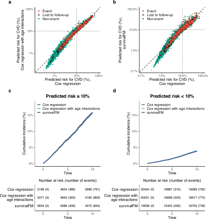
a Reclassification plot comparing individual risk predictions when adding QRISK3 age interaction terms to a standard Cox regression model (y-axis) versus a standard Cox model (x-axis). b Reclassification plot comparing risk predictions from survivalFM (y-axis) to the standard Cox model (x-axis). Both axes are on a log scale. Black dotted vertical and horizontal lines show the 10% absolute risk threshold for the high risk category. c Kaplan–Meier curves for cumulative CVD incidence in the high-risk group (≥10% predicted risk) across three models: (1) Cox regression (dark gray), (2) Cox regression with QRISK3 age interactions (light blue), and (3) survivalFM (blue), with a risk table below. d Kaplan–Meier analysis for the low-risk group (<10% predicted risk) using the same models and color coding. Results are based on the Scotland test set (N = 25,572, 1583 events). Source data are provided as a Source Data file.
To further assess model performance, we conducted a Kaplan–Meier analysis, evaluating observed CVD event risk over 10 years in patients stratified by the guideline recommended 10% risk threshold (Fig. 5c, d). As expected, cumulative event rates in these groups were consistent across models, reflecting both the shared 10% threshold and the fact that all models were well-calibrated (Supplementary Fig. 17a). Specifically, event rates were 15% in the high-risk group and 4% in the low-risk group across all models, with no significant differences in Kaplan–Meier curves (log-rank test: p = 0.88 for predicted risk ≥10%, p = 0.63 for predicted risk <10%). However, models incorporating interaction terms identified larger high-risk groups while maintaining comparable absolute risk thresholds, thereby capturing more events. By 10 years, survivalFM identified 844 events in the high-risk group (predicted risk ≥10%), a 6.7% increase over the 791 events captured by the standard Cox model. Adding QRISK3’s age interactions resulted in 809 events in the high-risk group, a smaller 2.3% increase over the standard Cox model.
Analysis of the model coefficients from survivalFM revealed a broad array of interactions contributing to the CVD predictions. The ratio of total cholesterol to HDL cholesterol demonstrated one of the most pronounced interaction profiles among all predictor variables (Fig. 6). This suggests that the effect of the cholesterol ratio on CVD risk is influenced by the presence of other risk factors. For example, the interaction weight for the cholesterol ratio with prevalent atrial fibrillation was negative, despite both factors having positive individual weights. This suggests that these variables capture partly overlapping aspects of cardiovascular risk. Atrial fibrillation is often associated with a broader cardiovascular risk36, which could already be reflected in the elevated cholesterol ratio. This may thus imply that when both risk factors are present, they do not independently add to the risk. Comparing the estimated effects for the model terms overlapping between survivalFM and the standard Cox regression model with linear and age interaction terms from QRISK3, the shared terms exhibited very similar weights, with correlation of 0.95 between the estimated effects by the two methods (Supplementary Fig. 18). This shows that despite the introduction of complex interactions, the fundamental risk associations remain broadly consistent.
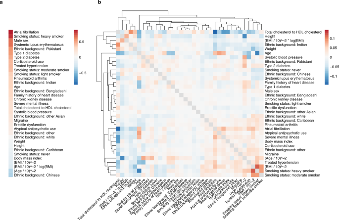
Estimated coefficients for a the linear effects β and b the interaction effects given by the inner product of the factor vectors βi,j = 〈pi, pj〉. The dendrogram shows a hierarchical clustering of the interaction profiles, using Euclidean distance as the measure of similarity. Source data are provided as a Source Data file.