Material
This study used a publicly accessible stroke datasetFootnote 1. The data set is inpatient and includes 12 different attributes of 5,110 patients. By reducing the aim examined in this study to a binary classification problem, this dataset identifies the target as stroke. A total of 5110 patients were assessed of which 4869 were patients without a stroke and 249 were patients with a stroke. There were 201 missing values for the “bmi” feature. For continuous variables, the median was employed to impute missing values since it is robust to outliers. The table1 describes the features of the dataset.
Data-set pre-processing
The purpose of data preparation is to make raw data more usable and comprehensible. Raw datasets provide several issues, including defects, erratic behavior, missing values, and inconsistency. Preprocessing is essential to solve missing data and gaps16. To get the dataset ready for deployment, it will require some pre-processing. Here, it has been replaced by the mean of the ’bmi’ feature, as many values are missing in this feature. Violin plots are used as an effective visualization method in ML, enabling the comprehension of data distribution across categories or classes by integrating comprehensive distribution information with essential summary statistics. The violin plot for features for instance age, average glucose level, and smoking status is shown in the Fig. 1. The violin plot (a) indicates that individuals who have a stroke are mostly older, exhibiting a greater density in the senior age demographic (60+ years). The age distribution for those without a stroke is broader, including all age groups, however, it is more concentrated in the middle age range of 40 to 50 years. Age is a crucial determinant of stroke risk. The narrative indicates that strokes are more prevalent among older adults, corroborating medical evidence that age is a significant risk factor for strokes. Plot (b) compares glucose levels between stroke survivors and non-stroke individuals. The no-stroke group has glucose levels between 80-130 mg/dL, while stroke survivors have a broader distribution, with a higher median glucose level. The plot suggests elevated glucose levels may increase the risk of stroke. The heart_disease plot (c) reveals a strong correlation between hypertension and stroke, with a higher proportion of individuals with hypertension in the stroke group and most non-stroke individuals not having hypertension. This highlights the significant risk factors for stroke. Plot (d) compares hypertension in stroke and non-stroke individuals. Stroke individuals have a higher proportion of hypertension, indicating a significant association between hypertension and stroke occurrence. Non-stroke individuals have a majority without hypertension. The findings suggest older age, higher average glucose levels, and hypertension are more common in stroke patients.

The violin plot for each feature of (a) age (b) avg_glucose_level (c)heart_disease (d) hypertension.
All correlation values in the dataset represent how much each feature is related to the target variable, which is stroke. Strong positive correlations indicate an increase in stroke likelihood, while weak or no linear relationships suggest a decrease. Gender has a very low positive correlation, suggesting that there is no linear relationship with the likelihood of stroke. Age has a moderate positive correlation, suggesting that older individuals are more likely to have a stroke. Hypertension has a low positive correlation, while heart disease has a low positive correlation. Ever married has a low positive correlation, suggesting some association with stroke risk. Work type has a very weak negative correlation, suggesting a slight inverse relationship with stroke likelihood. Residence type has a very weak positive correlation, with no linear relationship between location and stroke occurrence. Average glucose levels have a low positive correlation, and BMI has a very weak positive correlation. Smoking status has a very weak positive correlation, but it is still a known risk factor for stroke through its effects on cardiovascular health. The features with the highest correlation to stroke are age, hypertension, heart disease, and average glucose level.
Figure2 shows the variations of the features in correlation with the target variable, stroke. While 183 individuals did not have hypertension but did have a stroke, 4429 patients did not have either condition. 66 individuals suffered from both hypertension and stroke and 432 suffered from hypertension alone. While 4,632 individuals did not suffer from either heart disease or stroke, 202 people had the former but did not have the latter. At the same time, 229 people had heart disease but did not suffer from stroke, whereas 47 patients had both conditions. A total of 141 female patients had a stroke, while 2853 females did not. Similarly, 108 males experienced a stroke, whereas 2007 males remained stroke-free. Furthermore, 1497 patients with unknown smoking status did not have a stroke, while 47 patients with the same status did. Among individuals who had previously smoked, 70 experienced strokes, while 815 did not. Additionally, 90 people who had never smoked suffered strokes, whereas 1802 non-smokers remained stroke-free. Furthermore, 42 current smokers experienced strokes compared to 747 smokers who did not.

The bar plot for each feature of (a) age (b) avg_glucose_level (c) heart_disease (d) hypertension.
After data visualization and analysis, we split the data set into 70:20:10 for Training, validation, and Testing, respectively. In this preprocessing pipeline, missing values in the Body Mass Index (BMI) feature are imputed using the mean value strategy, computed solely from the training subset to prevent data leakage. This ensures consistency and robustness across validation and test sets. Subsequently, categorical variables namely( gender, ever_married, work_type, Residence_type, and smoking_status) are encoded using one hot encoding via Scikitlearn’s OneHotEncoder, configured to ignore unknown categories during transformation. The encoder is fitted exclusively on the training data to preserve the integrity of the validation and test datasets. The encoded categorical features are then transformed into individual binary indicator variables for each category, facilitating their compatibility with a wide range of machine learning algorithms. These steps represent a standard but essential part of the preprocessing pipeline, aimed at preparing both numerical and categorical data for downstream modeling while minimizing bias and ensuring reproducibility.
We evaluated six imbalance-handling methods(SMOTE, ADASYN, Hybrid Sampling, Threshold Moving, Cost-Sensitive Learning, and Two-Stage Classifiers) using F1-score and recall to assess their ability to mitigate class imbalance in the training dataset. As shown in Table2, Threshold Moving achieved the highest recall (0.76) among data-level techniques, coupled with a moderate F1-score (0.50) and low complexity, indicating a better trade-off between sensitivity and precision. SMOTE and ADASYN yielded lower recall scores (0.65 and 0.64, respectively) and low F1-scores (0.42 and 0.41) due to elevated false positive rates, while Hybrid Sampling slightly improved both recall (0.67) and F1-score (0.48), though at a higher computational cost.
Among model-level methods, Cost-Sensitive Learning delivered a balanced performance with high recall (0.75) and the highest F1-score (0.52), suggesting its effectiveness in handling class imbalance while preserving generalization. Notably, the Two-Stage Classifier achieved the highest recall (0.80) but suffered from lower accuracy (0.60) and increased complexity, potentially limiting its practical use in real-time clinical applications.
Overall, the results demonstrate that Threshold Moving, by adjusting the classifier’s decision boundary without altering the training data distribution, offers a practical and interpretable solution. It improves the classifier’s responsiveness to minority class instances (stroke cases) with minimal sacrifice to overall accuracy (0.70), resulting in a model that may be more applicable for future clinical investigations, pending further validation. As supported by Chicco and Jurman (2020)17, the F1-score is a more informative metric than accuracy in imbalanced biomedical datasets, and our findings confirm that model-level strategies such as Threshold Moving or Cost-Sensitive Learning are more effective than traditional resampling in optimizing both precision and recall critical metrics in high-stakes decision-making like stroke prediction.
Despite implementing several traditional imbalance-handling methods such as SMOTE, ADASYN, and Hybrid Sampling, many models exhibited relatively low F1-scores. This limitation is largely due to the highly skewed distribution of the dataset (249 stroke vs. 4861 non-stroke cases), which makes it challenging for classifiers to achieve a proper balance between precision and recall.
To address this, we conducted an expanded evaluation using the following strategies:
-
SMOTE, ADASYN, Hybrid Sampling, and Threshold Moving: Traditional data-level methods used to balance the class distribution.
-
Cost-Sensitive Learning: Incorporating class weights into classifiers (e.g., XGBoost, RandomForest) to penalize minority-class errors.
-
Two-Stage Classifiers: A sequential classification scheme where the first model filters potential positive cases and a second model refines predictions.
The comparative results across multiple criteria are summarized in Table 2.
Key observations from the table:
-
Best for Recall: Two-Stage Classifier, achieving recall of 0.80.
-
Best F1 Balance: Cost-Sensitive Learning, offering good recall with manageable complexity.
-
Best Lightweight Option: Threshold Moving, improving recall without additional data generation.
These findings confirm that no single method excels across all evaluation aspects. Instead, the strategy should be tailored to the objective of the study, be it improving sensitivity, maintaining generalization, or balancing complexity.
Feature selection
In order to choose the most relevant characteristics, this research used six feature selection methods (Pearson’s correlation, mutual information (MI), particle swarm optimization (PSO), chi-squared test, ANOVA F-test and Harris Hawks Optimization (HHO)), which contributed to the extraction of key features of the data set. The implementation of this methods facilitates better detection of which key indicators are linked to stroke occurrences. Multiple statistical analyses including Pearson’s correlation alongside the chi-squared test with the ANOVA F-test reveal different linear and non-linear associations between the target outcome and its features. The optimization approaches like PSO and HHO contribute to finding the best sets of features that enhance model performance.
Pearson’s correlation
We started by using Pearson’s correlation coefficient as our baseline statistical approach to measure linear associations between variables and stroke affect. The analysis benefited from Pearson’s correlation even though it only detects linear relationships because one-hot encoding was used on categorical values before preprocessing. The data transformation enabled full application of Pearson’s method to all variables. There are nonetheless unknown non-linear patterns that could exist and potential future analysis should explore such relationships with mutual information and tree-based importance assessment methods.
Figure 3 illustrates the Pearson correlation matrix among all features. This is an analysis of the principal elements in the correlation matrix. Pearson’s Correlation Coefficient measures the linear relationship between two variables, ranging from -1 to 1. A value of 1 indicates a perfect positive correlation, where both variables increase together, while -1 signifies a perfect negative correlation, where an increase in one variable corresponds to a decrease in the other. Linear association between variables stands weak when the correlation value approaches zero. The color gradient in the presented correlation matrix shows the relationship strength between variables through different shades where strong positive relationships appear in dark red and strong negative relationships appear in dark blue. The correlational relationship shows a complete negative alignment (-1) that exists between ever_married_No and ever_married_Yes together with smoking_status_smokes and smoking_status_never smoked because the data contains binary code categorizations. The data indicates that individuals who never worked tend to avoid working as government employees (-0.66). The analyses show light positive relationships exist between employees working for the government and non-smokers (0.24) and workers who never conducted employment and non-smokers (0.13). The two relationships connecting ever_married_No with work_type_Govt_job and Residence_type_Rural with smoking_status_smokes show negative weak strength (-0.17 for each). The majority of correlations involving gender_Male rate almost zero which shows minimal linear dependency exists. Tests conducted for variable correlations validated the feature selection procedures thus confirming that selected variables are fit for use in predictive modeling. The weak connections between features minimize both model stability problems and simplify interpretation of model results. For instance, the observed correlation of 0.68 between age and marital status (ever_married) reflects typical demographic patterns, where older individuals are more likely to be married. This supports the validity of the dataset’s structure and enhances trust in the correlations observed. Furthermore, even the modest positive correlations between stroke and variables such as age, hypertension, and heart disease align with well-established clinical risk factors, highlighting their relevance in stroke risk assessment.

A matrix representing Pearson’s correlation.
Stroke has modest relationships with many parameters, including age (0.25), hypertension (0.13), and heart disease (0.13), these factors show modest statistical associations with stroke occurrence. Although these correlations are modest, they confirm known risk factors for stroke. This highlights the importance of considering these factors in predictive models.
Mutual Information (MI)
In feature selection, the Mutual Information is a common method18. The concept of Mutual Information from information theory provides a measurement tool to evaluate the information content about a variable that one variable contains regarding another. In the context of machine learning and feature selection, MI measures the dependency between a feature and the target variable. The Results of categorized according to their contribution to the target variable, shown in Table5 and Fig. 4.

Comparison top feature importance between Mutual Information (MI) and randomforest classifier.
Particle Swarm Optimization (PSO)
The Particle Swarm Optimization (PSO) technique was used for optimizing feature selection for the dataset. The objective function assessed the performance of the feature subset, while PSO was set with using 5-fold cross-validation, a swarm size of 20 and a maximum of 30 iterations. Upon reaching the iteration limit, the ideal feature subset was identified based on the highest particle weights, with features with a weight of 0.5 or more being chosen.
The PSO optimization achieved a maximum score of 0.92. The chosen collection of characteristics include [’heart_disease’, ’avg_glucose_level’, ’gender_Male’, ’gender_Other’, ’work_type_Never_worked’, ’work_type_Private’, ’work_type_Selfemployed’, ’work_type_children’, ’Residence_type_Rural’, ’Residence_type_Urban’, ’smoking_status_Unknown’, ’smoking_status_formerly smoked’, ’smoking_status_never smoked’, ’smoking_status_smokes’]. This feature set is anticipated to enhance the model’s performance substantially.
Chi-squared test
Based on primary data and the model’s assumptions, a statistical test will be selected. Rather, in the context of an experiment with a binary result, classification is relevant, and the chi-square test is also applicable in the training data when examining the dependence of categorical features on the target variable. Table3 displays the results of the Chi-squared statistics. P-value measures the probability of obtaining the Chi-squared score if we assume that the null hypothesis (the feature and the target do not have any relationship between them) is true. A low p-value (generally< 0.05) signifies a statistically significant relationship between the trait and the target variable.
Work_type has the maximum Chi-square score with a value of 171.921085 and a p-value approaching zero ( 2.815761e-39 ). So, there is a really strong relation between work_type and the target variable and it is really unlikely to be coincidence. Residence_type has Chi-square: 86.297855, p-value: 1.547763e-20, this is yet another very good sign for the target. Ever_married has a Chi-squared score: of 61.766296, p-value: 3.867376e-15, this feature also correlates strongly with the target. Smoking status has a Chi-squared score of 54.952606 and a p-value of 1.234716e-13. It also has a strong link to the aim based on statistics. Heart disease shows a Chi-squared score of 11.677804 and a p-value of 6.325014e-04. While important (p-value< 0.05), this trait’s link to the aim isn’t as strong as the ones we talked about before. Hypertension has a Chi-squared score of 0.538132 and a p-value of 0.4632078. The high p-value tells us there is no real tie between hypertension and what we are looking at.
Features that have high Chi-squared scores and low p-values (such as work_type and Residence_type) tend to play a bigger role in predicting the target variable. However, traits with low scores and high p-values (such as hypertension) may not add much value. You could think of leaving these out or giving them less attention when you analyze data or build models later on.
ANOVA F-test statistics
The ANOVA F-test (Analysis Of Variance F-test) can be adopted as a statistic that tests the null hypothesis to establish whether there is a significant difference in the means of two or more groups. In ML, it is applied to measure the relationship between a set of numerical variables and one categorial variable19. Amongst the numerical features, age has the highest correlation coefficient, and average glucose level and BMI occupy the second and third positions respectively. All three features are significant at the P-value level of significance However, if you have to just choose between the three, you might need to go with the numerical features, especially, the age and avg_glucose_level for feature engineering or modeling as table4 show.
Harris Hawks Algorithm (HHO)
Employs Harris Hawks Optimization (HHO) to identify the most important features for a classification model. The objective function evaluates feature subsets by converting weights into binary selections and using a Random Forest classifier to measure their performance through 5-fold cross-validation. The HHO algorithm initializes the hawks (candidate solutions) and iteratively updates their positions to minimize the negative accuracy score, aiming to find the optimal feature subset. The HHO optimization achieved a maximum score of 0.8740. The chosen collection of featurers include [’age’, ’heart_disease’, ’avg_glucose_level’, ’gender_Male’, ’gender_Other’, ’ever_married_Yes’, ’work_type_Govt_job’, ’work_type_Selfemployed’, ’Residence_type_Rural’, ’smoking_status_Unknown’, ’smoking_status_never smoked’].
According to the previous analysis, the main factors that show statistical association with stroke, as identified by the applied feature selection algorithms, are shown in the following table 5, which compares the methods applied.
Summary of results by feature selection method most top feature importance depending out the feature selection methods that applied in this study is shown in the Fig. 5

A matrix representing Pearson’s correlation.
Proposed algorithms
The ML workflow includes steps such as preparing and selecting data, choosing an appropriate model, training it, evaluating its performance, and finally deploying the model. Iterative testing and fine-tuning are frequently used to boost model performance. The ultimate goal is to build a model that generalizes well to new data and successfully addresses the specific problem.
The selection of the ideal model relies heavily on hyperparameter tuning. During hyperparameter selection, we want to focus on the good results of earlier rounds of training. Improving the model is made easier by adjusting the algorithms parameters20.In this work, we utilized a Nested Cross-Validation strategy combined with manual grid search to optimize the hyperparameters optimization approach. The inner loop of the nested CV was used for model tuning by systematically evaluating predefined combinations of hyperparameters (such as the number of hidden units, dropout rate, and learning rate), while the outer loop provided an unbiased evaluation of the model’s generalization performance. This approach ensures robust and reliable hyperparameter selection while avoiding overfitting. Grid search is a tuning technique that performs an exhaustive parameter search by systematically evaluating each value inside the designated hyperparameter space. Various methodologies exist for using ML ensemble models, such as boosting, stacking, and bagging. Using applied ensemble learning, we combine several individual models to produce more accurate predictions than a single model alone.
To prevent data leakage and ensure the correctness of measures of performance, all data balancing techniques (SMOTE, ADASYN, Hybrid Sampling, and Cost-Sensitive Learning) were only used in the training datasets in each cross-validation iteration. In each iteration of each fold of the nested cross-validation only the training subsets were affected by resampling and weight class while the validation/test data were kept untouched throughout. This approach ensures that synthetic samples or class distributions do not leak into the validation or testing phases, thereby providing an unbiased estimate of model generalizability.
Traditional machine learning model training
Several machine learning models receive training through a reliable nested cross-validation strategy that uses both robust evaluation and prevention of overfitting. The models consist of Logistic Regression along with Random Forest and XGBoost along with Support Vector Machine (SVM) and K-Nearest Neighbors (KNN). The optimization process for hyperparameters applies GridSearchCV methodology on 3-fold inner cross-validation followed by a generalization assessment through 5-fold outer cross-validation for each model. The F1-score together with AUC and Precision, Recall and Accuracy represent the evaluation metrics used. A StackingClassifier joins the pipeline by uniting different base models (RandomForest and SVM and XGBoost) whose final prediction stems from a meta-model (Logistic Regression). The ensemble technique uses multiple classifiers to enhance predictive ability through their distinctive contribution to the results. The models save their evaluation results to enable a comparative study which correlated with selecting the most successful prediction method.
Deep Neural Network (DNN) training
A Deep Neural Network (DNN) was designed through an implementation that integrated nested cross-validation to optimize hyperparameters while maintaining unbiased performance assessment. After the input layer the DNN contains one hidden layer with 64 or 128 neurons based on configuration while using ReLU activation functions. The dropout layer contains a drop rate of 0.3 or 0.5 to minimize overfitting effects. One neuron with a sigmoid activation function exists within the output layer to perform binary classification tasks. The model employed Adam optimization at learning rates of 0.001 and 0.0001 while using the binary cross-entropy loss function. The training process lasted 10 epochs under 32 batch processing conditions. The inner loop part of nested cross-validation (3-fold CV) used a grid search technique which selected the best hyperparameter set through optimization of F1-score performance. The best model chosen during the 5-fold CV process received further training before assessment with outside test data. Averaged F1-score together with standard deviation metrics of Accuracy, Precision, Recall and AUC were reported for the final model evaluation across all outer cross-validation splits.
For the evaluation of each model on the test set, accuracy, and classification reports including precision, recall, and F1-score are computed. For the DNN, the outputs are thresholded at 0.5 to produce 0/1 labels as seen above, which is not the case with other models. The metrics for each model at different classes are presented by a confusion matrix shown in the form of heatmaps which provide a clear image of the true positive, false positive, true negatives, and false negatives. It also has a functionality to compare models where it prints out accuracy scores and provides a brief idea about how well any of the models are classifying the test data.
The outcomes achieved by the models were analyzed about the dataset through the application of XAI approaches. The three XAI models applied in this study are:
-
SHAP (SHapley Additive exPlanations): is a model agnostic approach to assess the output of any ML model by quantifying the significance of each feature in relation to the final prediction.
-
LIME (Local Interpretable Model-agnostic Explanations): is a way to approximate black-box models with interpretable models trained on subsets of data in order to generate local interpretations of those models.
-
ELI5 (Explain Like I’m 5): is a Python library that makes it easy to understand ML models. It explains how the models work using methods like showing which features are most important, visualizing decision trees, and analyzing how shuffling features affect predictions.
-
PDP (Partial Dependence Plot): is a global explainable AI (XAI) technique used to visualize the marginal effect of one or two features on the predicted outcome of a machine learning model. It shows how the prediction changes as a selected feature changes, while averaging out the effects of all other features in the dataset.
An ML architecture is a sequence of connected and compatible data processing components whereby the entire workflow of an ML work is automated. Normally, it deals with the preparation of data, feature engineering, model selection, adjustment of hyperparameters, and an assessment of its performance. It is designed to effectively enhance the efficiency of ML models through a systematic and automated approach across the whole process. Figure 6 illustrates the ML architecture used in the research.
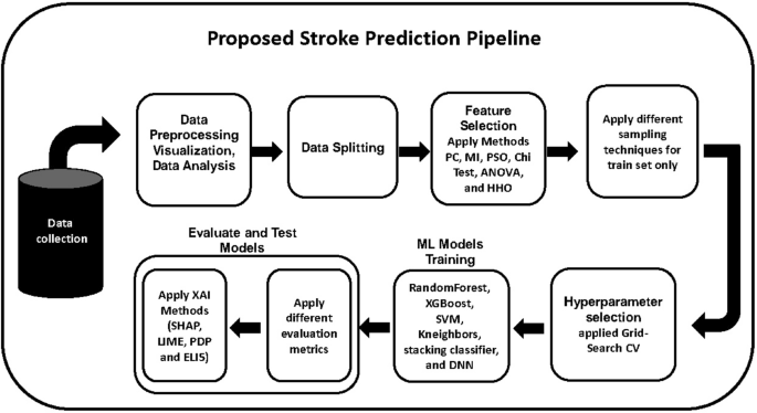
the workflow design for proposed machine learning pipeline.
